Survival curves

This function produces Kaplan-Meier plots using ggplot2. As a first argument it needs a survfit object, created by the survival package. Default settings differ for single stratum and multiple strata objects.

Usage

ggsurv(
  s,
  CI = "def",
  plot.cens = TRUE,
  surv.col = "gg.def",
  cens.col = "gg.def",
  lty.est = 1,
  lty.ci = 2,
  size.est = 0.5,
  size.ci = size.est,
  cens.size = 2,
  cens.shape = 3,
  back.white = FALSE,
  xlab = "Time",
  ylab = "Survival",
  main = "",
  order.legend = TRUE
)

Arguments

s

an object of class survfit

CI

should a confidence interval be plotted? Defaults to TRUE for single stratum objects and FALSE for multiple strata objects.

plot.cens

mark the censored observations?

surv.col

colour of the survival estimate. Defaults to black for one stratum, and to the default ggplot2 colours for multiple strata. Length of vector with colour names should be either 1 or equal to the number of strata.

cens.col

colour of the points that mark censored observations.

lty.est

linetype of the survival curve(s). Vector length should be either 1 or equal to the number of strata.

lty.ci

linetype of the bounds that mark the 95% CI.

size.est

line width of the survival curve

size.ci

line width of the 95% CI

cens.size

point size of the censoring points

cens.shape

shape of the points that mark censored observations.

back.white

if TRUE the background will not be the default grey of ggplot2 but will be white with borders around the plot.

xlab

the label of the x-axis.

ylab

the label of the y-axis.

main

the plot label.

order.legend

boolean to determine if the legend display should be ordered by final survival time

Value

An object of class ggplot

Author

Edwin Thoen

Examples

# Small function to display plots only if it's interactive
p_ <- GGally::print_if_interactive

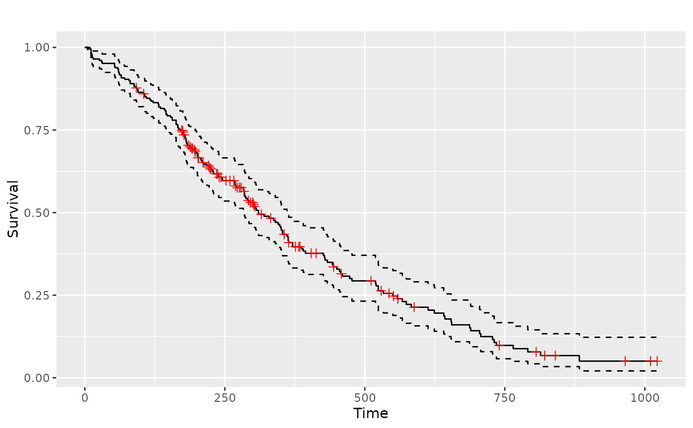
if (require(survival) && require(scales)) {
  lung <- survival::lung
  sf.lung <- survival::survfit(Surv(time, status) ~ 1, data = lung)
  p_(ggsurv(sf.lung))

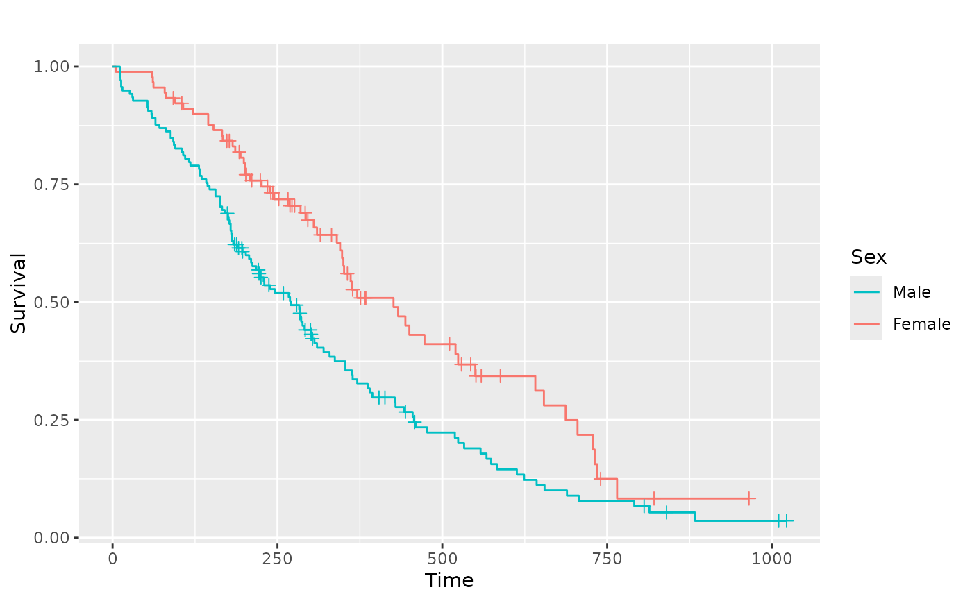
  # Multiple strata examples
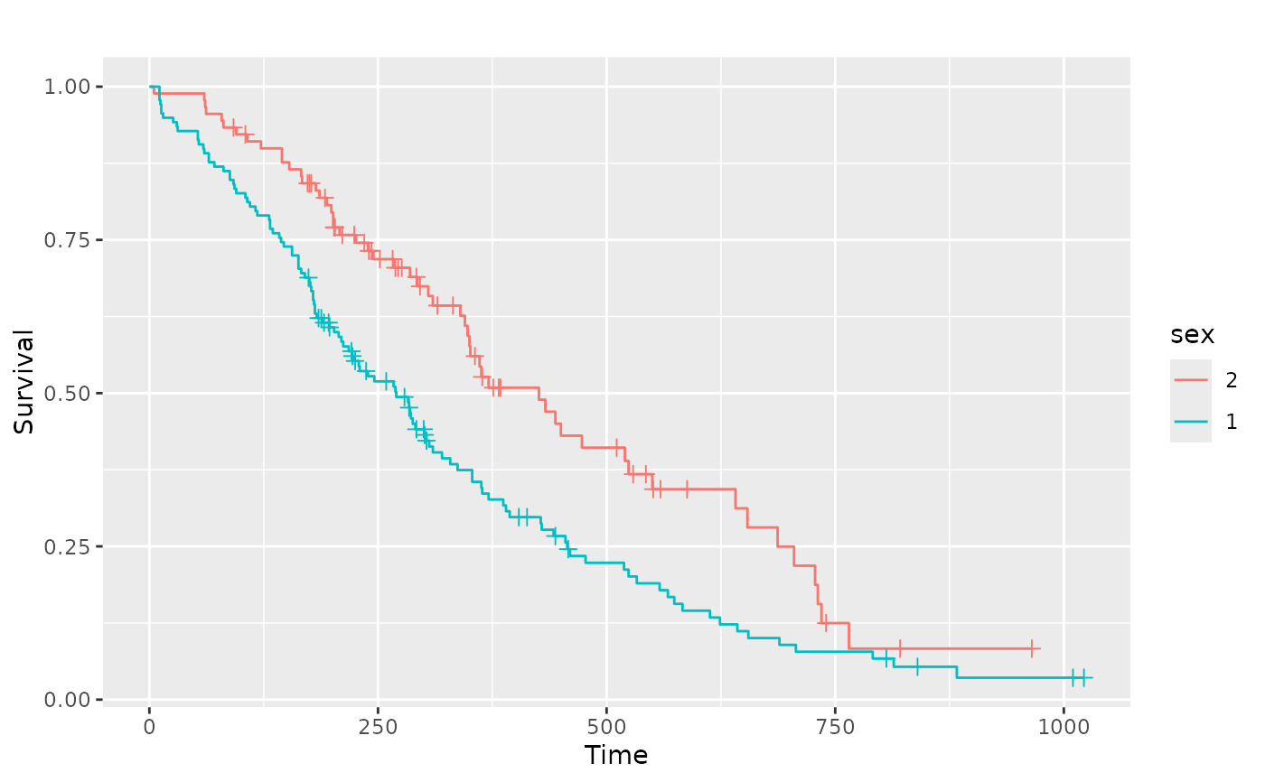
  sf.sex <- survival::survfit(Surv(time, status) ~ sex, data = lung)
  pl.sex <- ggsurv(sf.sex)
  p_(pl.sex)

  # Adjusting the legend of the ggsurv fit
  p_(pl.sex +
    ggplot2::guides(linetype = "none") +
    ggplot2::scale_colour_discrete(
      name   = "Sex",
      breaks = c(1, 2),
      labels = c("Male", "Female")
    ))

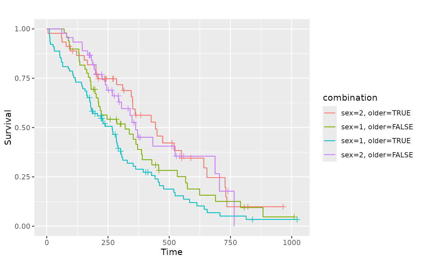
  # Multiple factors
  lung2 <- dplyr::mutate(lung, older = as.factor(age > 60))
  sf.sex2 <- survival::survfit(Surv(time, status) ~ sex + older, data = lung2)
  pl.sex2 <- ggsurv(sf.sex2)
  p_(pl.sex2)

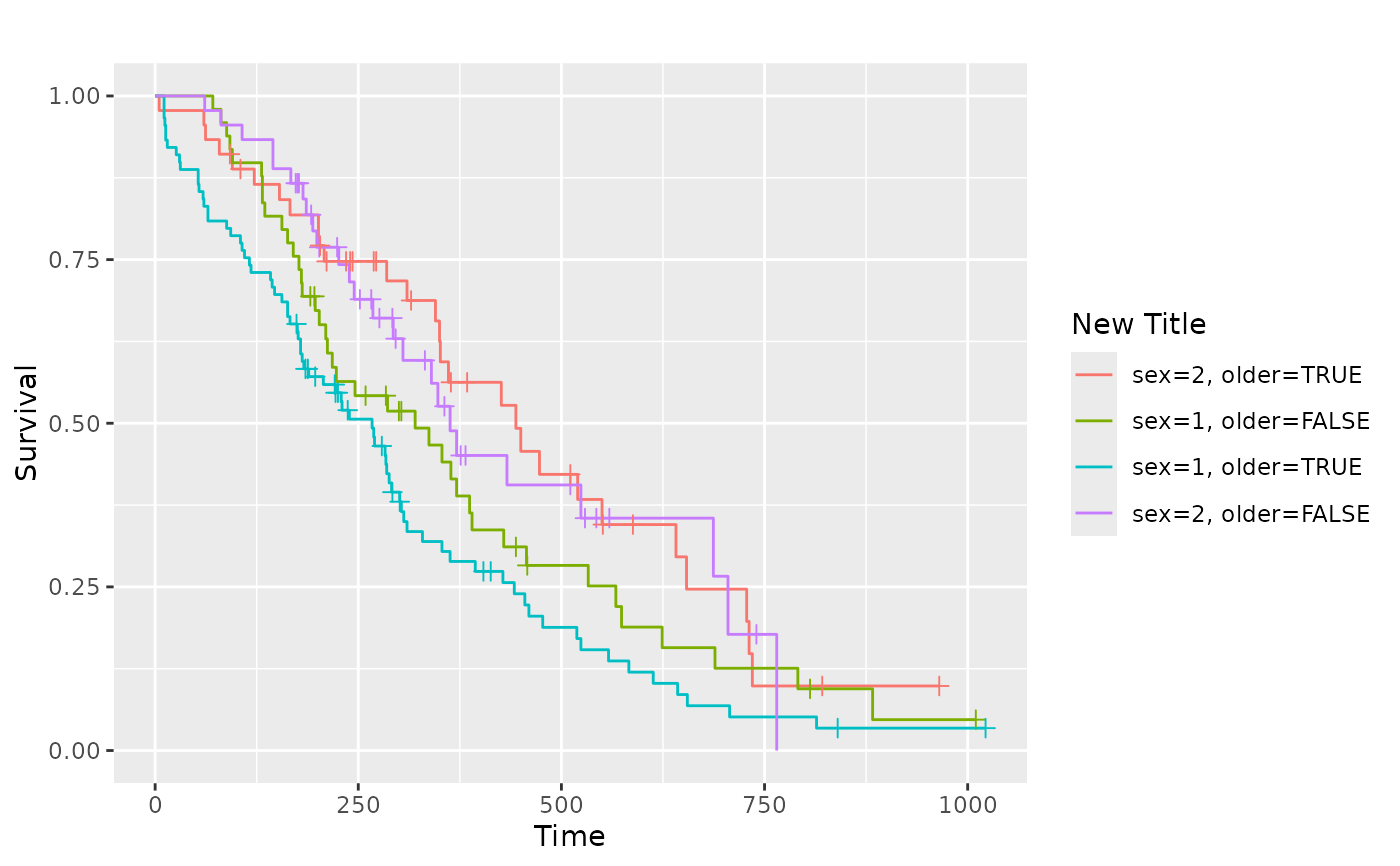
  # Change legend title
  p_(pl.sex2 + labs(color = "New Title", linetype = "New Title"))

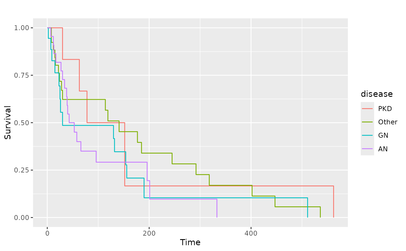
  # We can still adjust the plot after fitting
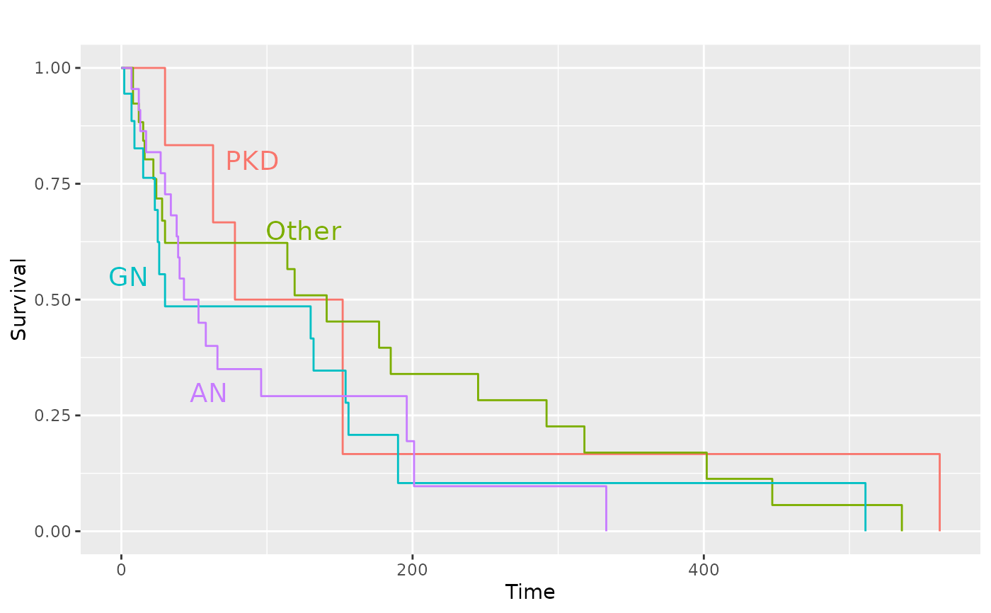
  kidney <- survival::kidney
  sf.kid <- survival::survfit(Surv(time, status) ~ disease, data = kidney)
  pl.kid <- ggsurv(sf.kid, plot.cens = FALSE)
  p_(pl.kid)

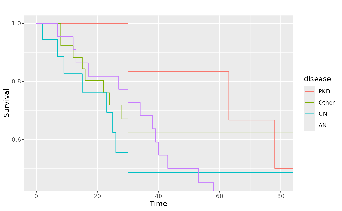
  # Zoom in to first 80 days
  p_(pl.kid + ggplot2::coord_cartesian(xlim = c(0, 80), ylim = c(0.45, 1)))

  # Add the diseases names to the plot and remove legend
  p_(pl.kid +
    ggplot2::annotate(
      "text",
      label = c("PKD", "Other", "GN", "AN"),
      x = c(90, 125, 5, 60),
      y = c(0.8, 0.65, 0.55, 0.30),
      size = 5,
      colour = scales::pal_hue(
        h         = c(0, 360) + 15,
        c         = 100,
        l         = 65,
        h.start   = 0,
        direction = 1
      )(4)
    ) +
    ggplot2::guides(color = "none", linetype = "none"))
}
#> Loading required package: survival
#> Loading required package: scales


#> Scale for colour is already present.
#> Adding another scale for colour, which will replace the existing
#> scale.