ggpairs(): Pairwise plot matrix

library(GGally)
#> Loading required package: ggplot2
#> Registered S3 method overwritten by 'GGally':
#>   method from   
#>   +.gg   ggplot2

`GGally::ggpairs()`

ggpairs() is a special form of a ggmatrix() that produces a pairwise comparison of multivariate data. By default, ggpairs() provides two different comparisons of each pair of columns and displays either the density or count of the respective variable along the diagonal. With different parameter settings, the diagonal can be replaced with the axis values and variable labels.

There are many hidden features within ggpairs(). Please take a look at the examples below to get the most out of ggpairs().

Columns and Mapping

The columns displayed default to all columns of the provided data. To subset to only a few columns, use the columns parameter.

data(tips)
pm <- ggpairs(tips)
pm
#> `stat_bin()` using `bins = 30`. Pick better value with `binwidth`.
#> `stat_bin()` using `bins = 30`. Pick better value with `binwidth`.
#> `stat_bin()` using `bins = 30`. Pick better value with `binwidth`.
#> `stat_bin()` using `bins = 30`. Pick better value with `binwidth`.
#> `stat_bin()` using `bins = 30`. Pick better value with `binwidth`.
#> `stat_bin()` using `bins = 30`. Pick better value with `binwidth`.
#> `stat_bin()` using `bins = 30`. Pick better value with `binwidth`.
#> `stat_bin()` using `bins = 30`. Pick better value with `binwidth`.
#> `stat_bin()` using `bins = 30`. Pick better value with `binwidth`.
#> `stat_bin()` using `bins = 30`. Pick better value with `binwidth`.
#> `stat_bin()` using `bins = 30`. Pick better value with `binwidth`.
#> `stat_bin()` using `bins = 30`. Pick better value with `binwidth`.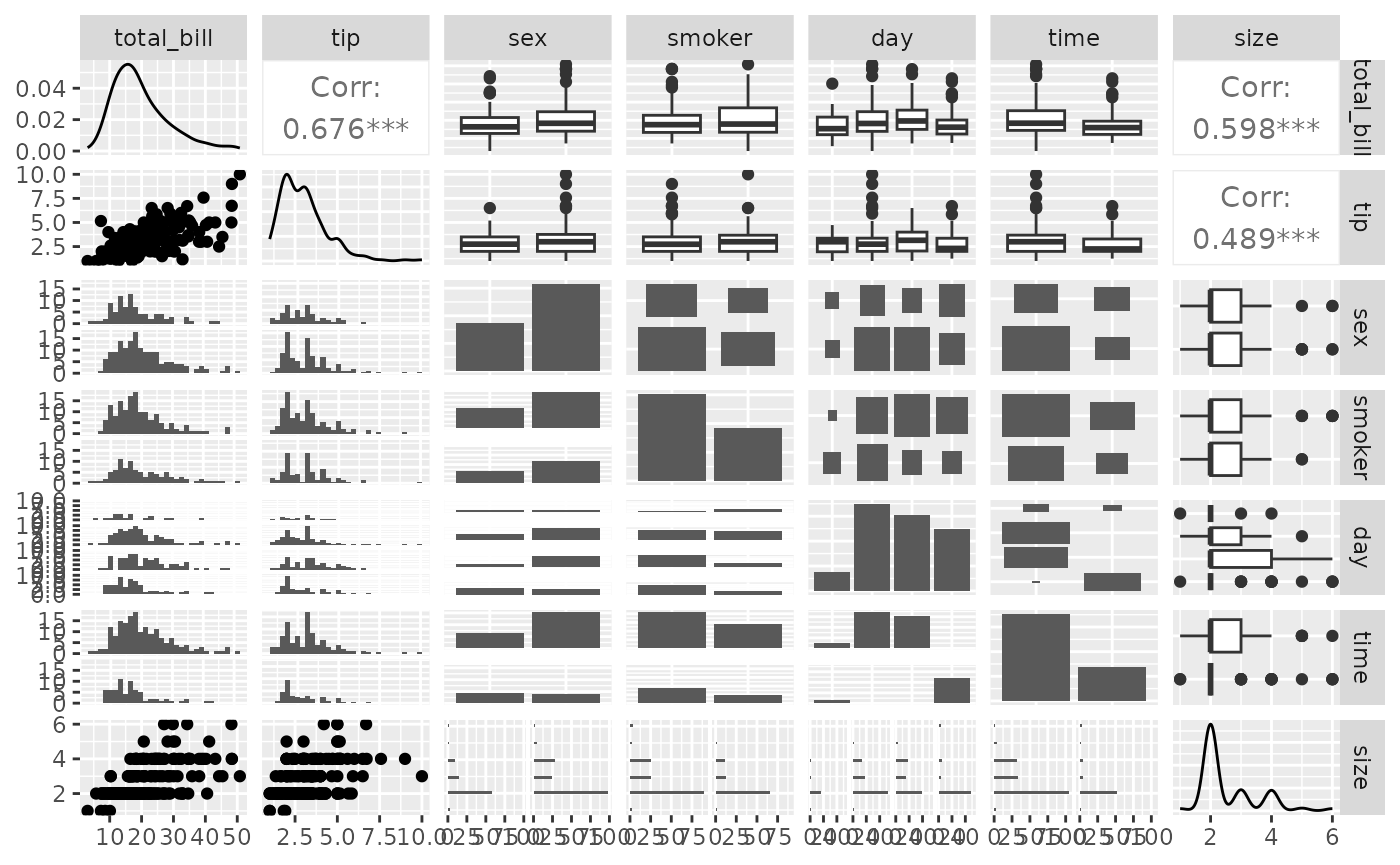

## too many plots for this example.

## reduce the columns being displayed
## these two lines of code produce the same plot matrix
pm <- ggpairs(tips, columns = c(1, 6, 2))
pm <- ggpairs(tips, columns = c("total_bill", "time", "tip"), columnLabels = c("Total Bill", "Time of Day", "Tip"))
pm
#> `stat_bin()` using `bins = 30`. Pick better value with `binwidth`.
#> `stat_bin()` using `bins = 30`. Pick better value with `binwidth`.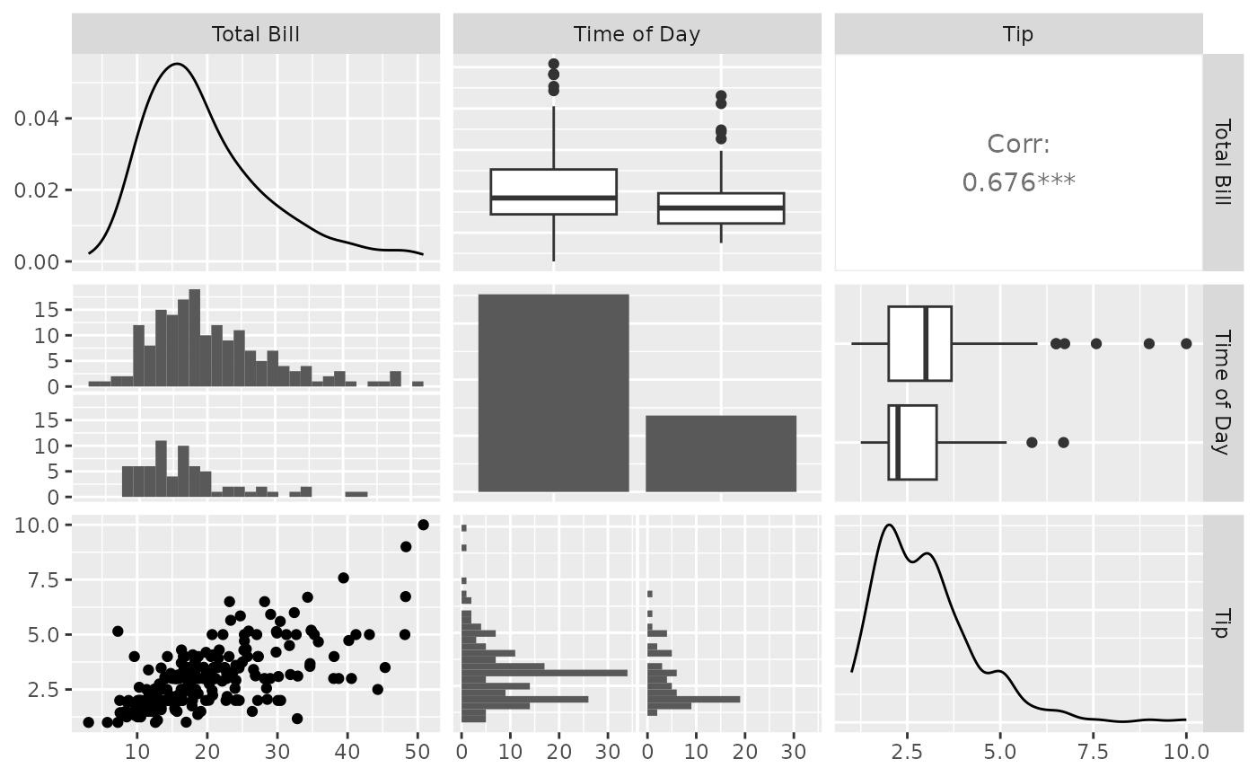

Aesthetics can be applied to every subplot with the mapping parameter.

library(ggplot2)
pm <- ggpairs(tips, mapping = aes(color = sex), columns = c("total_bill", "time", "tip"))
pm
#> `stat_bin()` using `bins = 30`. Pick better value with `binwidth`.
#> `stat_bin()` using `bins = 30`. Pick better value with `binwidth`.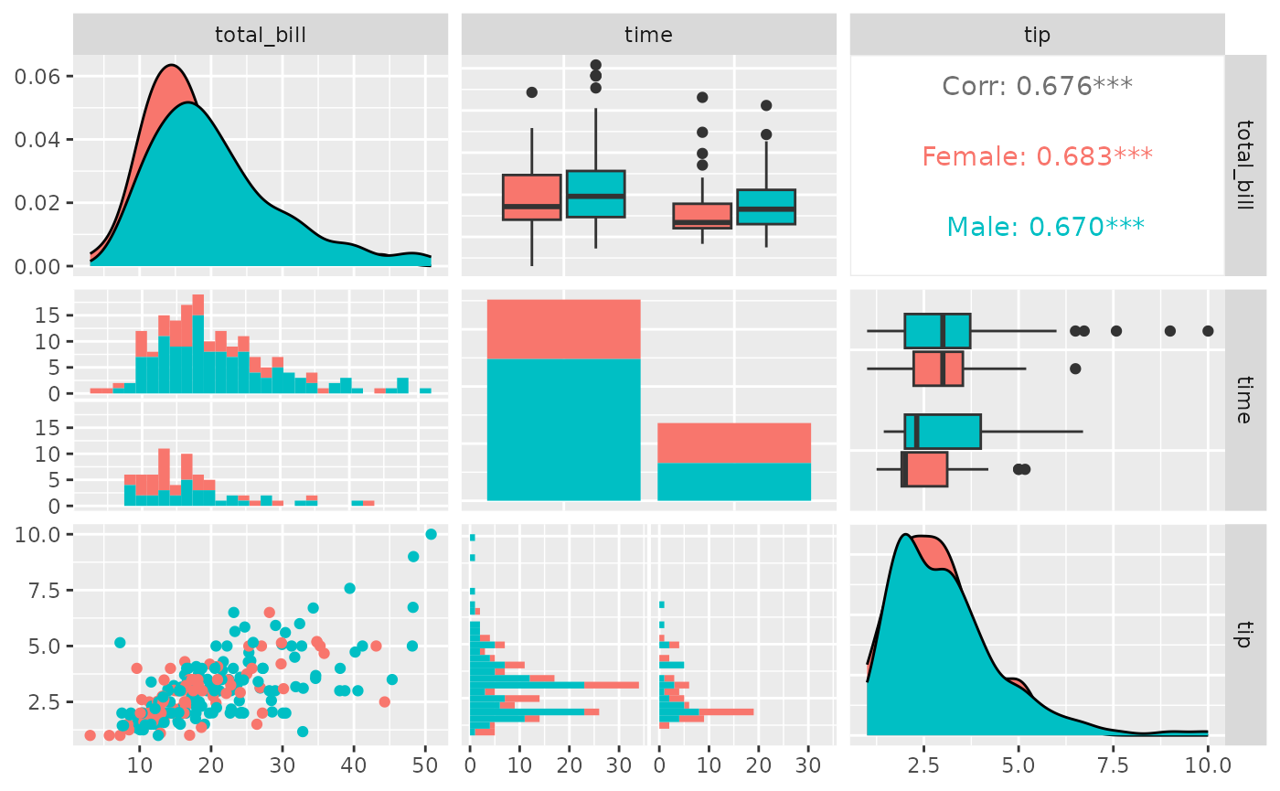

Since the plots are default plots (or are helper functions from GGally), the aesthetic color is altered to be appropriate. Looking at the example above, ‘tip’ vs ‘total_bill’ (pm[3,1]) needs the color aesthetic, while ‘time’ vs ‘total_bill’ needs the fill aesthetic. If custom functions are supplied, no aesthetic alterations will be done.

Matrix Sections

There are three major sections of the pairwise matrix: lower, upper, and diag. The lower and upper may contain three plot types: continuous, combo, and discrete. The ‘diag’ only contains either continuous or discrete.

continuous: both X and Y are continuous variables
combo: one X and Y variable is discrete while the other is continuous
discrete: both X and Y are discrete variables

To make adjustments to each section, a list of information may be supplied. The list can be comprised of the following elements:

continuous: a character string representing the tail end of a ggally_NAME function, or a custom function
combo: a character string representing the tail end of a ggally_NAME function, or a custom function. (not applicable for a diag list)
discrete: a character string representing the tail end of a ggally_NAME function, or a custom function
mapping: if mapping is provided, only the section’s mapping will be overwritten

The list of current valid ggally_NAME functions is visible in vig_ggally("ggally_plots").

library(ggplot2)
pm <- ggpairs(
  tips,
  columns = c("total_bill", "time", "tip"),
  lower = list(
    continuous = "smooth",
    combo = "facetdensity",
    mapping = aes(color = time)
  )
)
pm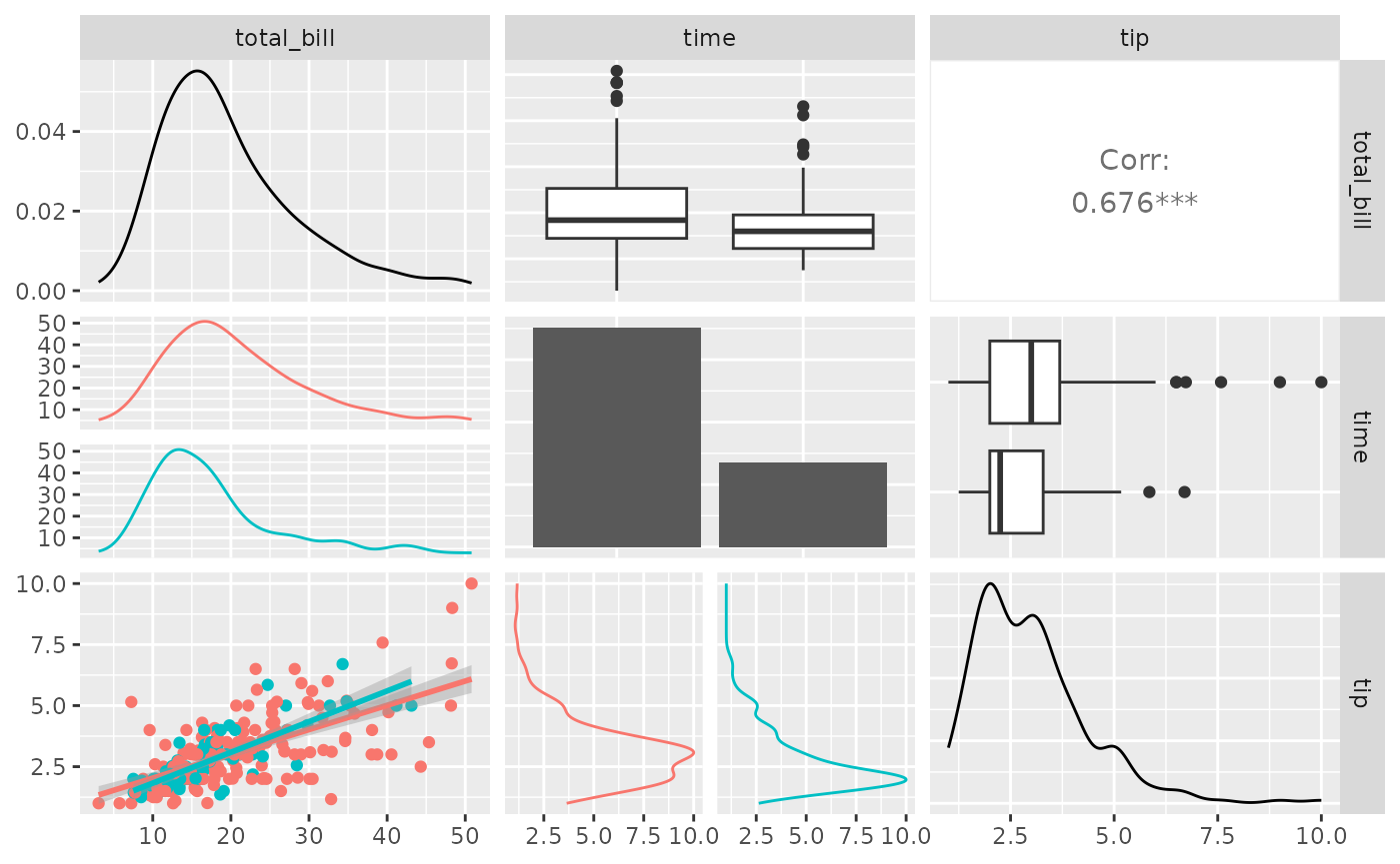

A section list may be set to the character string "blank" or NULL if the section should be skipped when printed.

pm <- ggpairs(
  tips,
  columns = c("total_bill", "time", "tip"),
  upper = "blank",
  diag = NULL
)
pm
#> `stat_bin()` using `bins = 30`. Pick better value with `binwidth`.
#> `stat_bin()` using `bins = 30`. Pick better value with `binwidth`.

Custom Functions

The ggally_NAME functions do not provide all graphical options. Instead of supplying a character string to a continuous, combo, or discrete element within upper, lower, or diag, a custom function may be given.

The custom function should follow the api of

custom_function <- function(data, mapping, ...) {
  # produce ggplot2 object here
}

There is no requirement to what happens within the function, as long as a ggplot2 object is returned.

my_bin <- function(data, mapping, ..., low = "#132B43", high = "#56B1F7") {
  ggplot(data = data, mapping = mapping) +
    geom_bin2d(...) +
    scale_fill_gradient(low = low, high = high)
}
pm <- ggpairs(
  tips,
  columns = c("total_bill", "time", "tip"),
  lower = list(
    continuous = my_bin
  )
)
pm
#> `stat_bin()` using `bins = 30`. Pick better value with `binwidth`.
#> `stat_bin()` using `bins = 30`. Pick better value with `binwidth`.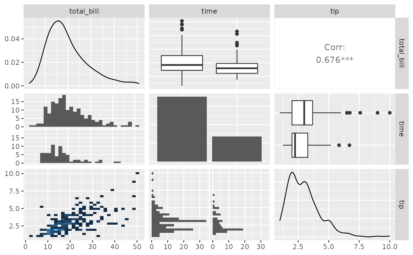

Function Wrapping

The examples above use default parameters to each of the subplots. One of the immediate parameters to be set it binwidth. This parameters is only needed in the lower, combination plots where one variable is continuous while the other variable is discrete.

To change the default parameter binwidth setting, we will wrap() the function. wrap() first parameter should be a character string or a custom function. The remaining parameters supplied to wrap will be supplied to the function at run time.

pm <- ggpairs(
  tips,
  columns = c("total_bill", "time", "tip"),
  lower = list(
    combo = wrap("facethist", binwidth = 1),
    continuous = wrap(my_bin, binwidth = c(5, 0.5), high = "red")
  )
)
pm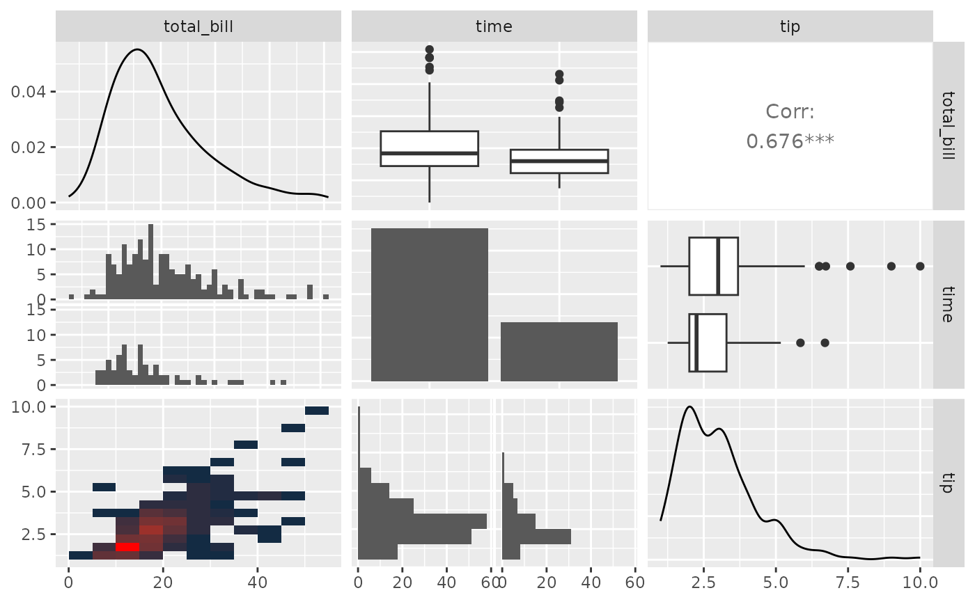

To get finer control over parameters, please look into custom functions.

Plot Matrix Subsetting

Please look at the vignette for ggmatrix on plot matrix manipulations.

Small ggpairs() example:

pm <- ggpairs(tips, columns = c("total_bill", "time", "tip"))
# retrieve the third row, first column plot
p <- pm[3, 1]
p <- p + aes(color = time)
p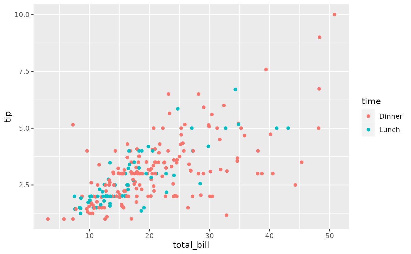

pm[3, 1] <- p
pm
#> `stat_bin()` using `bins = 30`. Pick better value with `binwidth`.
#> `stat_bin()` using `bins = 30`. Pick better value with `binwidth`.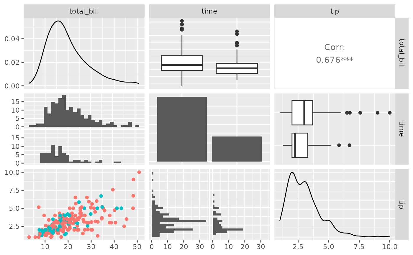

Themes

Please look at the vignette for ggmatrix on plot matrix manipulations.

Small ggpairs() example:

pmBW <- pm + theme_bw()
pmBW
#> `stat_bin()` using `bins = 30`. Pick better value with `binwidth`.
#> `stat_bin()` using `bins = 30`. Pick better value with `binwidth`.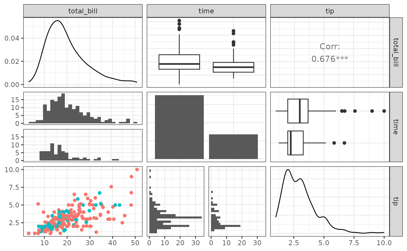

References

John W Emerson, Walton A Green, Barret Schloerke, Jason Crowley, Dianne Cook, Heike Hofmann, Hadley Wickham. The Generalized Pairs Plot. Journal of Computational and Graphical Statistics, vol. 22, no. 1, pp. 79-91, 2012.

Barret Schloerke

Oct 29, 2015

GGally::ggpairs()