ggnostic(): Model diagnostics

library(GGally)
#> Loading required package: ggplot2
#> Registered S3 method overwritten by 'GGally':
#>   method from   
#>   +.gg   ggplot2

`GGally::ggnostic()`

ggnostic() is a display wrapper to ggduo() that displays full model diagnostics for each given explanatory variable. By default, ggduo() displays the residuals, leave-one-out model sigma value, leverage points, and Cook’s distance against each explanatory variable. The rows of the plot matrix can be expanded to include fitted values, standard error of the fitted values, standardized residuals, and any of the response variables. If the model is a linear model, stars are added according to the stats::anova significance of each explanatory variable.

Most diagnostic plots contain reference line(s) to help determine if the model is fitting properly

residuals:
- Type key: ".resid"
- A solid line is located at the expected value of 0 with dashed lines at the 95% confidence interval. (\(0 \pm 1.96 * \sigma\))
- Plot function: ggally_nostic_resid().
- See also stats::residuals
standardized residuals:
- Type key: ".std.resid"
- Same as residuals, except the standardized residuals equal the regular residuals divided by sigma. The dashed lines are located at \(0 \pm 1.96 * 1\).
- Plot function: ggally_nostic_std_resid().
- See also stats::rstandard
leave-one-out model sigma:
- Type key: ".sigma"
- A solid line is located at the full model’s sigma value.
- Plot function: ggally_nostic_sigma().
- See also stats::influence’s value on sigma
leverage points:
- Type key: ".hat"
- The expected value for the diagonal of a hat matrix is \(p / n\). Points are considered leverage points if they are large than \(2 * p / n\), where the higher line is drawn.
- Plot function: ggally_nostic_hat().
- See also stats::influence’s value on hat
Cook’s distance:
- Type key: ".cooksd"
- Points that are larger than \(4 / n\) line are considered highly influential points. Plot function: ggally_nostic_cooksd(). See also stats::cooks.distance()
fitted points:
- Type key: ".fitted"
- No reference lines by default.
- Default plot function: ggally_points().
- See also stats::predict
standard error of fitted points:
- Type key: ".se.fit"
- No reference lines by default.
- Plot function: ggally_nostic_se_fit().
- See also stats::fitted
response variables:
- Type key: (response name in data.frame)
- No reference lines by default.
- Default plot function: ggally_points().

Life Expectancy Model Fitting

Looking at the dataset datasets::state.x77, we will fit a multiple regression model for Life Expectancy.

# make a data.frame and fix column names
state <- as.data.frame(state.x77)
colnames(state)[c(4, 6)] <- c("Life.Exp", "HS.Grad")
str(state)
#> 'data.frame':    50 obs. of  8 variables:
#>  $ Population: num  3615 365 2212 2110 21198 ...
#>  $ Income    : num  3624 6315 4530 3378 5114 ...
#>  $ Illiteracy: num  2.1 1.5 1.8 1.9 1.1 0.7 1.1 0.9 1.3 2 ...
#>  $ Life.Exp  : num  69 69.3 70.5 70.7 71.7 ...
#>  $ Murder    : num  15.1 11.3 7.8 10.1 10.3 6.8 3.1 6.2 10.7 13.9 ...
#>  $ HS.Grad   : num  41.3 66.7 58.1 39.9 62.6 63.9 56 54.6 52.6 40.6 ...
#>  $ Frost     : num  20 152 15 65 20 166 139 103 11 60 ...
#>  $ Area      : num  50708 566432 113417 51945 156361 ...

# fit full model
model <- lm(Life.Exp ~ ., data = state)
# reduce to "best fit" model with
model <- step(model, trace = FALSE)
summary(model)
#> 
#> Call:
#> lm(formula = Life.Exp ~ Population + Murder + HS.Grad + Frost, 
#>     data = state)
#> 
#> Residuals:
#>      Min       1Q   Median       3Q      Max 
#> -1.47095 -0.53464 -0.03701  0.57621  1.50683 
#> 
#> Coefficients:
#>               Estimate Std. Error t value Pr(>|t|)    
#> (Intercept)  7.103e+01  9.529e-01  74.542  < 2e-16 ***
#> Population   5.014e-05  2.512e-05   1.996  0.05201 .  
#> Murder      -3.001e-01  3.661e-02  -8.199 1.77e-10 ***
#> HS.Grad      4.658e-02  1.483e-02   3.142  0.00297 ** 
#> Frost       -5.943e-03  2.421e-03  -2.455  0.01802 *  
#> ---
#> Signif. codes:  0 '***' 0.001 '**' 0.01 '*' 0.05 '.' 0.1 ' ' 1
#> 
#> Residual standard error: 0.7197 on 45 degrees of freedom
#> Multiple R-squared:  0.736,  Adjusted R-squared:  0.7126 
#> F-statistic: 31.37 on 4 and 45 DF,  p-value: 1.696e-12

Next, we look at the variables for any high (|value| > 0.8) correlation values and general interaction behavior.

# look at variables for high correlation (none)
ggscatmat(state, columns = c("Population", "Murder", "HS.Grad", "Frost"))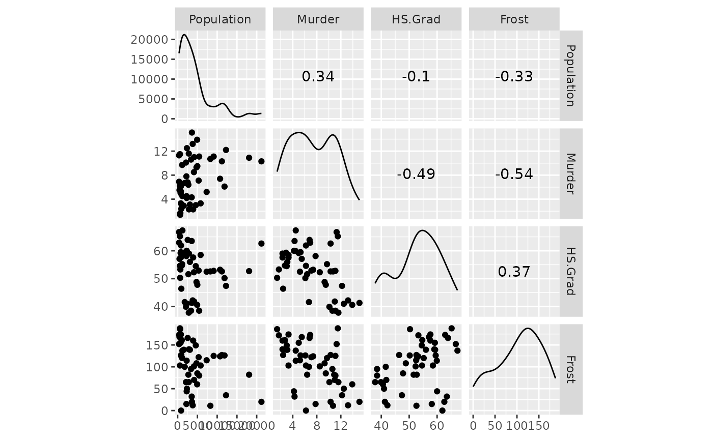

All variables appear to be ok. Next, we look at the model diagnostics.

# look at model diagnostics
ggnostic(model)
#> `geom_smooth()` using method = 'loess'
#> `geom_smooth()` using method = 'loess'
#> `geom_smooth()` using method = 'loess'
#> `geom_smooth()` using method = 'loess'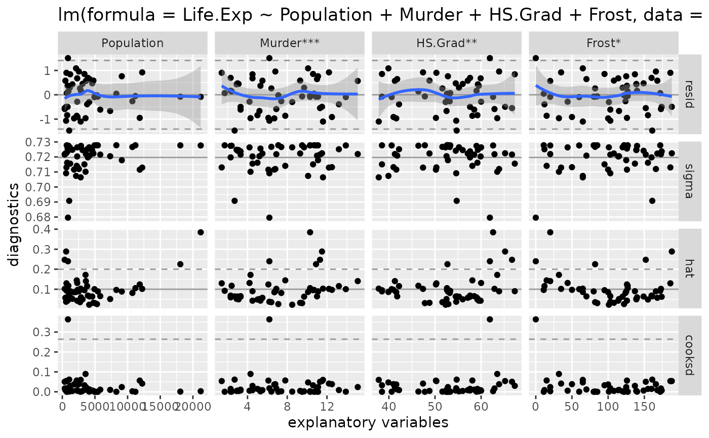

The residuals appear to be normally distributed. There are a couple residual outliers, but 2.5 outliers are expected.
There are 5 leverage points according the diagonal of the hat matrix
There are 2 leverage points according to Cook’s distance. One is much larger than the other.

Let’s remove the largest data point first to try and define a better model.

# very high life expectancy
state[11, ]
#>        Population Income Illiteracy Life.Exp Murder HS.Grad Frost Area
#> Hawaii        868   4963        1.9     73.6    6.2    61.9     0 6425
state_no_hawaii <- state[-11, ]
model_no_hawaii <- lm(Life.Exp ~ Population + Murder + HS.Grad + Frost, data = state_no_hawaii)
ggnostic(model_no_hawaii)
#> `geom_smooth()` using method = 'loess'
#> `geom_smooth()` using method = 'loess'
#> `geom_smooth()` using method = 'loess'
#> `geom_smooth()` using method = 'loess'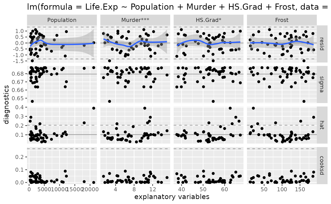

There are no more outrageous Cook’s distance values. The model without Hawaii appears to be a good fitting model.

summary(model)
#> 
#> Call:
#> lm(formula = Life.Exp ~ Population + Murder + HS.Grad + Frost, 
#>     data = state)
#> 
#> Residuals:
#>      Min       1Q   Median       3Q      Max 
#> -1.47095 -0.53464 -0.03701  0.57621  1.50683 
#> 
#> Coefficients:
#>               Estimate Std. Error t value Pr(>|t|)    
#> (Intercept)  7.103e+01  9.529e-01  74.542  < 2e-16 ***
#> Population   5.014e-05  2.512e-05   1.996  0.05201 .  
#> Murder      -3.001e-01  3.661e-02  -8.199 1.77e-10 ***
#> HS.Grad      4.658e-02  1.483e-02   3.142  0.00297 ** 
#> Frost       -5.943e-03  2.421e-03  -2.455  0.01802 *  
#> ---
#> Signif. codes:  0 '***' 0.001 '**' 0.01 '*' 0.05 '.' 0.1 ' ' 1
#> 
#> Residual standard error: 0.7197 on 45 degrees of freedom
#> Multiple R-squared:  0.736,  Adjusted R-squared:  0.7126 
#> F-statistic: 31.37 on 4 and 45 DF,  p-value: 1.696e-12
summary(model_no_hawaii)
#> 
#> Call:
#> lm(formula = Life.Exp ~ Population + Murder + HS.Grad + Frost, 
#>     data = state_no_hawaii)
#> 
#> Residuals:
#>      Min       1Q   Median       3Q      Max 
#> -1.48967 -0.50158  0.01999  0.54355  1.11810 
#> 
#> Coefficients:
#>               Estimate Std. Error t value Pr(>|t|)    
#> (Intercept)  7.106e+01  8.998e-01  78.966  < 2e-16 ***
#> Population   6.363e-05  2.431e-05   2.618   0.0121 *  
#> Murder      -2.906e-01  3.477e-02  -8.357 1.24e-10 ***
#> HS.Grad      3.728e-02  1.447e-02   2.576   0.0134 *  
#> Frost       -3.099e-03  2.545e-03  -1.218   0.2297    
#> ---
#> Signif. codes:  0 '***' 0.001 '**' 0.01 '*' 0.05 '.' 0.1 ' ' 1
#> 
#> Residual standard error: 0.6796 on 44 degrees of freedom
#> Multiple R-squared:  0.7483, Adjusted R-squared:  0.7254 
#> F-statistic: 32.71 on 4 and 44 DF,  p-value: 1.15e-12

Since there is only a marginal improvement by removing Hawaii, the original model should be used to explain life expectancy.

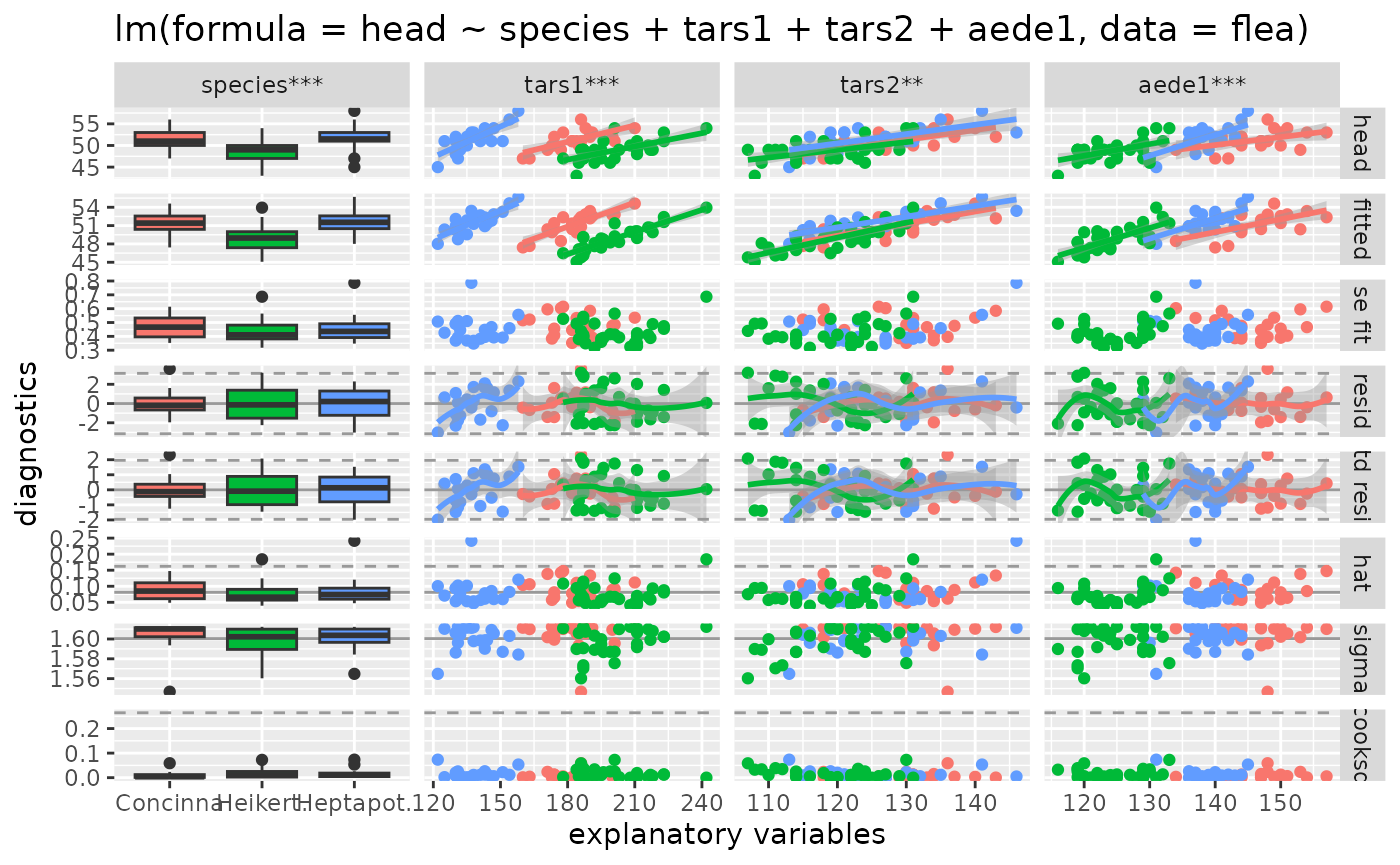
Full diagnostic plot matrix example

The following lines of code will display different model diagnostic plot matrices for the same statistical model. The first one is of the default settings. The second adds color according to the species. Finally, the third displays all possible columns and uses ggally_smooth() to display the fitted points and response variables.

flea_model <- step(lm(head ~ ., data = flea), trace = FALSE)
summary(flea_model)
#> 
#> Call:
#> lm(formula = head ~ species + tars1 + tars2 + aede1, data = flea)
#> 
#> Residuals:
#>     Min      1Q  Median      3Q     Max 
#> -3.0152 -1.2315 -0.0048  1.1490  3.6068 
#> 
#> Coefficients:
#>                  Estimate Std. Error t value Pr(>|t|)    
#> (Intercept)       0.63693    6.09162   0.105 0.917034    
#> speciesHeikert.   1.13651    1.25452   0.906 0.368171    
#> speciesHeptapot.  5.22207    0.92110   5.669 3.18e-07 ***
#> tars1             0.06815    0.01989   3.426 0.001043 ** 
#> tars2             0.10160    0.03297   3.081 0.002974 ** 
#> aede1             0.17069    0.04275   3.993 0.000163 ***
#> ---
#> Signif. codes:  0 '***' 0.001 '**' 0.01 '*' 0.05 '.' 0.1 ' ' 1
#> 
#> Residual standard error: 1.6 on 68 degrees of freedom
#> Multiple R-squared:  0.685,  Adjusted R-squared:  0.6618 
#> F-statistic: 29.57 on 5 and 68 DF,  p-value: 7.997e-16
# default output
ggnostic(flea_model)
#> `geom_smooth()` using method = 'loess'
#> `geom_smooth()` using method = 'loess'
#> `geom_smooth()` using method = 'loess'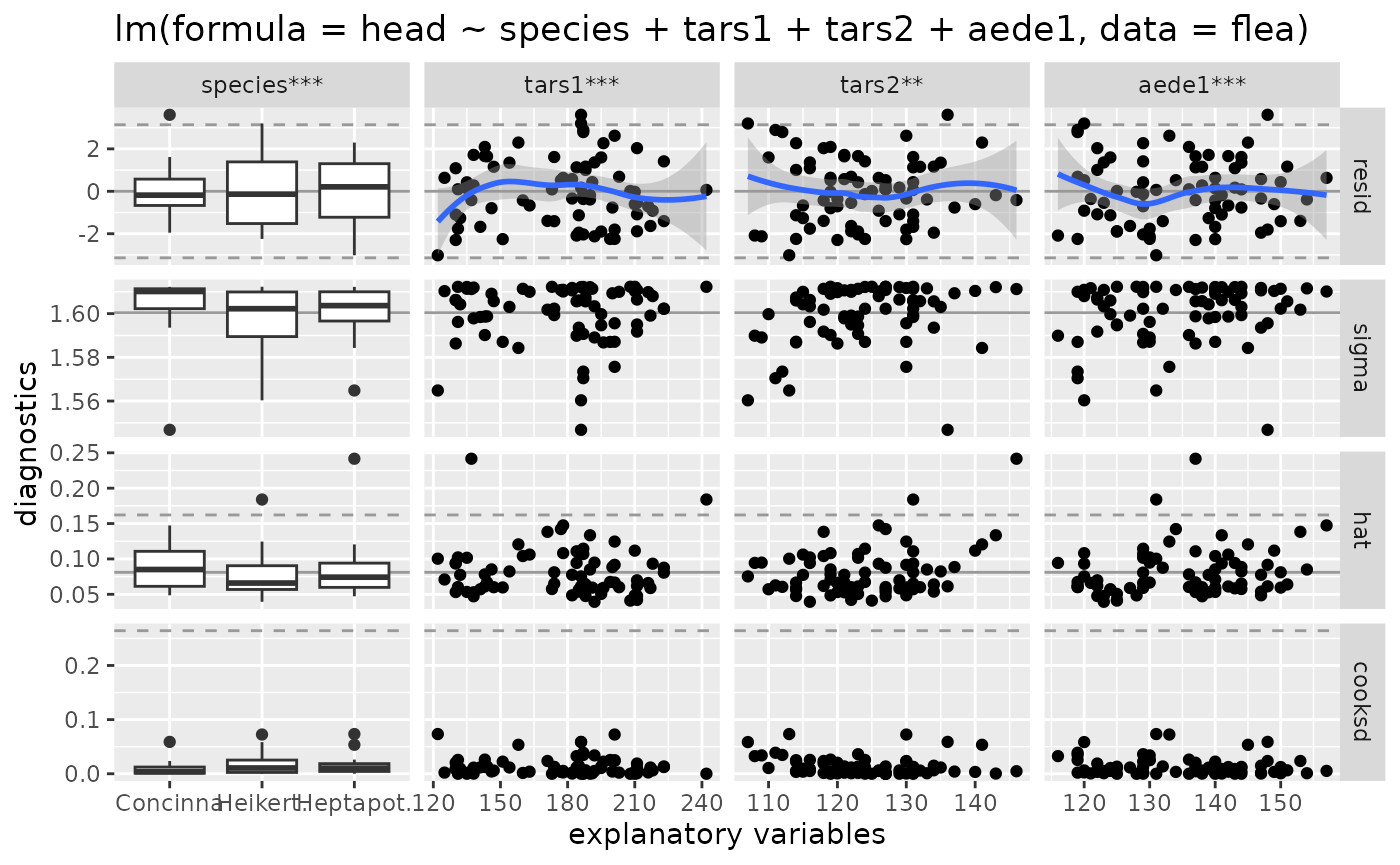

# color'ed output
ggnostic(flea_model, mapping = ggplot2::aes(color = species))
#> `geom_smooth()` using method = 'loess'
#> `geom_smooth()` using method = 'loess'
#> `geom_smooth()` using method = 'loess'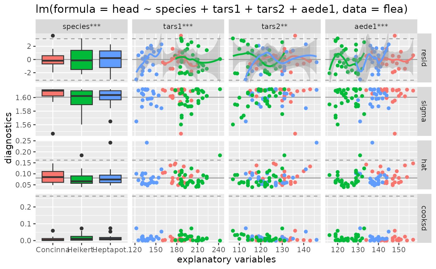

# full color'ed output
ggnostic(
  flea_model,
  mapping = ggplot2::aes(color = species),
  columnsY = c("head", ".fitted", ".se.fit", ".resid", ".std.resid", ".hat", ".sigma", ".cooksd"),
  continuous = list(default = ggally_smooth, .fitted = ggally_smooth)
)
#> `geom_smooth()` using method = 'loess'
#> `geom_smooth()` using method = 'loess'
#> `geom_smooth()` using method = 'loess'
#> `geom_smooth()` using method = 'loess'
#> `geom_smooth()` using method = 'loess'
#> `geom_smooth()` using method = 'loess'

Barret Schloerke

Oct 1, 2016

`GGally::ggnostic()`

Life Expectancy Model Fitting

Full diagnostic plot matrix example